C Transcriptomic cross-species analysis of chronic liver disease reveals consistent regulation between humans and mice

C.1 Supplementary Material and Methods

C.1.1 Collecting, curating, and processing publicly available genome-wide transcriptomics data

The raw data of the publicly available genome-wide transcriptomic studies (.CEL files for microarrays and count matrices for RNA-seq) were downloaded from Gene Expression Omnibus (GEO; Edgar et al. (2002)) and ArrayExpress (Kauffmann et al., 2009). For the respective accession, identifier see Table 4.1. Associated metadata was manually collected or accessed via the R/Bioconductor package GEOquery (version 2.56.0; S. Davis & Meltzer (2007)). To further process the raw data of microarrays and RNA-seq a suite of different Bioconductor packages (Gentleman et al., 2004) was used.

C.1.1.1 Processing of microarray data

First, a probe-level model was fitted to the raw data to subsequently control the array quality based on the relative log expression values (RLE) and the normalized unscaled standard errors (NUSE) using the R/Bioconductor package oligo (version 1.52.0; Carvalho & Irizarry (2010)). Arrays that deviated more than 0.1 from 0 for RLE and from 1 for NUSE were discarded due to expected poor quality. Subsequently, the raw data was normalized with the RMA algorithm, also implemented within the oligo package. Dependent on the studied organisms probe identifiers were mapped either to mouse/MGI or human/HGNC symbols using the R/Bioconductor package annotate (version 1.66.0) in combination with the individual annotation package of the used array type (e.g. hugene11sttranscriptcluster.db). If several probes matched the same gene symbol the expression was averaged. Genes with a constant expression across all samples were manually removed.

C.1.1.2 Processing of RNA-seq data

The preprocessing started by filtering out lowly expressed genes using the R/Bioconductor package edgeR (version 3.30.0; Robinson et al. (2010)) to increase the power of downstream statistical tests. Subsequently, the expression data was normalized by correcting for differences in library composition using also edgeR. Finally, the normalized data was transformed to log2-counts per million with the R/Bioconductor package limma (version 3.44.1; Ritchie et al. (2015))

C.1.2 Differential gene expression analysis

The differential gene expression analysis was performed using the R/Bioconductor package limma (version 3.44.1; Ritchie et al. (2015)). Unless otherwise stated a gene is considered differentially expressed with a false discovery rate (FDR) \(\le\) 0.05 and |logFC| \(\ge\) 1. Experiments with a time course or case-control design were handled differently. The resulting gene signatures of a differential gene expression analysis is referred to as contrast.

C.1.2.1 Time course design

For the acute CCl₄, Acetaminophen (APAP), and partial hepatectomy (PH) experiment, each time point is compared vs time point 0 to extract the effect of the respective intoxication or treatment. The chronic CCl₄ experiment was handled differently since time-matched oil controls were available for month 2 and month 12, but not for month 6 (Figure 4.1A). As the oil effect was assumed to be constant across time the expression values for the oil sample at month 6 were imputed by averaging the expression of the oil samples at month 2 and month 12. To regress out the effect of the oil the treated samples were compared against their time-matched oil controls. Also, the Bile duct ligation (BDL) experiment was handled differently because there were time-matched sham surgery samples available for days 1, 3, and 7 but not for day 21 (Supplementary Figure C.8A). For this reason, the expression values for the sham surgery sample at day 21 were again imputed by averaging the expression of the remaining sham surgery samples. Finally, the effect of BDL was extracted by comparing BDL samples vs time-matched sham surgery samples.

C.1.2.2 Case-Control design

For the experiments following the classical case-control design which is true for the Lipopolysaccharide (LPS) and Tunicamycin mouse models and all human studies, treated samples/patients with CLD were compared against untreated/healthy samples/patients or samples of patients with lower disease stages.

C.1.3 Clustering of time-series gene expression data

Time-series gene expression data were clustered with the software program STEM (Short Time-series Expression Miner, version 1.3.12; Ernst et al. (2005); Ernst & Bar-Joseph (2006)). As input, log-fold changes were provided from preceded differential gene expression analysis, where each time point was compared against time point 0. Accordingly, within STEM the normalization strategy “No normalization/add 0” was selected. Expression profiles were clustered using the default STEM clustering method with a specified maximal change between time points of 10 to not exclude drastic changes in the gene expression program, given partially large time spans between individual time points. Up to 20 different model profiles were returned by STEM. All other STEM parameters were left as default.

C.1.4 Comparing the similarity of gene sets via the Jaccard Index and Overlap Coefficient

The similarity or overlap between two gene sets was summarized either as Jaccard Index or Overlap Coefficient. Jaccard Index was used if the tested gene set had the same size, while for unbalanced gene set size the Overlap Coefficient was used. For the similarity analysis among the different acute mouse models or patient cohorts, the gene sets were composed of the top 500 differentially expressed genes based on limma’s moderated t-value.

C.1.5 Testing direction of regulation with Gene Set Enrichment Analysis

To test whether the differentially expressed genes of an arbitrary study A are consistently regulated in an also arbitrary but independent study B Gene Set Enrichment Analysis (GSEA; Subramanian et al. (2005)) was performed. From study A the top 500 up-and downregulated genes were extracted based on the moderated t-statistic. If the upregulated genes of study A are enriched among the upregulated genes of study B GSEA returns a positive enrichment score (ES). For enriched downregulated genes among the downregulated genes of study B a negative ES. GSEA was performed with the R/Bioconductor package fgsea (version 1.14.0; Sergushichev (2016)). If the enrichment was significant (FDR \(\le\) 0.05) it is concluded that either up- and/or downregulated genes of study A are consistently regulated also in study B.

C.1.6 Selection of the time point of the strongest altered expression profile

For the reversible acute time-course experiments (CCl₄, APAP, and BDL) the time point with the strongest deregulated expression profile was determined by comparing the mean distance of the individual time points to their respective control time point along with the principal component 1 (PC1) axis in the principal component (PC) space. The time point with the largest mean distance was considered as the time point of strongest deregulation. For the bile duct ligation experiment this strategy was not applicable due to the irreversible damage. We selected 24 hours as this was comparable to the selected time points of the other acute experiments.

C.1.7 Functional characterization of transcriptomic data with various gene set resources

To functionally characterize the mouse and human transcriptomic data sets different gene set resources were used, such as biological processes from Gene Ontology (GO (Ashburner et al., 2000)), DoRothEA’s regulons of confidence level A, B, and C (Garcia-Alonso et al., 2019; Christian H. Holland, Szalai, et al., 2020) and PROGENy’s top 100 pathway responsive-genes (Christian H. Holland, Szalai, et al., 2020; Schubert et al., 2018). GO gene sets were accessed with the R package msigdf (version 7.1; https://github.com/ToledoEM/msigdf), which queries itself the Molecular Signatures Database (MSigDB; Liberzon et al. (2011)). DoRothEA and PROGENy gene sets were accessed via their corresponding R/Bioconductor packages dorothea (version 1.0.1) and progeny (version 1.11.3).

As the statistical method overrepresentation analysis (ORA) was applied via the R function stats::fisher.test(). The number of background genes was set to 20,000 as this reflects a reasonable number of covered genes in transcriptomic studies. The minimum required gene set size was set to 10. The false discovery rate (FDR) is computed for each gene set resource individually to account for multiple hypothesis testing.

C.1.8 Manual clustering and text analysis of GO-terms

Significantly overrepresented GO-terms (FDR \(\le\) 0.05) were further analyzed by manual classification into more coarse-grained biological processes and text analysis to identify the most common keywords. Text analysis was performed with the R package tidytext (version 0.2.6; Silge & Robinson (2016)). Numbers and highly unspecific words such as “process” or “regulation” were removed. The frequencies of the most common keywords were visualized as word cloud with the R package ggwordcloud (version 0.5.0; https://lepennec.github.io/ggwordcloud/).

C.1.9 Construction and ranking of exclusive chronic, exclusive acute, and common gene sets

To identify a set of genes that is exclusive for chronic or acute liver damage in mouse models the acute and chronic mouse studies were integrated.

C.1.9.1 Construction of gene sets

First, the union of all differentially expressed genes was built across all the contrasts derived from the chronic or acute mouse experiment. A gene was considered differentially expressed with a FDR \(\le\) 1e-4 and |logFC| \(\ge\) 1. This conservative FDR threshold was opted for to include only the most reliable deregulated genes in this analysis. Indeed all chronic contrasts were considered. In the acute setup, however, the last time point of the bile duct ligation experiment (21 days after surgery) was removed as this damage is no longer considered to be acute. A consensus gene-level statistic was assigned for each gene in the unified chronic and acute gene set by computing the median of the t-statistics. Based on the sign of this consensus gene-level statistic genes were classified as up or downregulated. Genes that are listed only in the chronic or acute gene set were considered as exclusive chronic or exclusive acute genes, respectively. Accordingly, genes that were covered by both gene sets were deregulated in the liver irrespective of the nature of the damage. Therefore this gene set is referred to as the “common” gene set.

C.1.9.2 Ranking of gene sets

For these three different gene sets, a metric was computed per gene \(i\) integrating statistics from the chronic and selected acute contrasts. Regarding the acute mouse models, the number of considered acute contrasts was expanded. Next to the time points with the strongest deregulated profile, all time points between 8 and 48 hours were integrated to take into account the dynamic process of liver injury and recovery.

Metric for exclusive chronic gene set: i) consensus chronic gene-level statistic \(c_{consensus-chronic_{i\ }}\), ii) median t-statistic of selected acute contrasts \(\mu_{acute_{i\ }}\), and iii) variance of selected acute contrasts \(\sigma_{acute_{i\ }}^2\).

\[rank\left(\left|c_{consensus-chronic_{i\ }}\cdot\ \frac{1}{\mu_{acute_{i\ }}\ }\ \cdot\ \sqrt{\frac{1}{\sigma_{acute_{i\ }}^2}}\right|\right)\]

This metric prioritizes genes that have a high consensus chronic gene-level statistic and at the same time are consistently not deregulated in selected acute contrasts.

Metric for exclusive acute gene set: i) consensus acute gene-level statistic \(a_{consensus-acute_{i\ }}\), ii) median t-statistic of selected chronic contrasts \(\mu_{chronic_{i\ }}\) and iii) variance of selected chronic contrasts \(\sigma_{chronic_{i\ }}^2\).

\[rank\left(\left|a_{consensus-acute_{i\ }}\cdot\ \frac{1}{\mu_{chronic_{i\ }}\ }\ \cdot\ \sqrt{\frac{1}{\sigma_{chronic_{i\ }}^2}}\right|\right)\] Similar to above this metric ranks genes high that have a high consensus acute gene-level statistic and at the same time are consistently not deregulated in the chronic contrasts.

Metric for common gene set: same variables as for the exclusive chronic gene set.

\[rank\left(c_{consensus-chronic_{i\ }}\cdot\ \frac{1}{\mu_{acute_{i\ }}\ }\ \cdot\ \sqrt{\frac{1}{\sigma_{acute_{i\ }}^2}}\right)\]

This metric will rank genes high that have a high consensus chronic gene-level statistic and simultaneously are consistently and strongly regulated in the same direction as in the chronic scenario in selected acute contrasts.

C.1.10 Identification of consistently deregulated genes in patients and chronic CCl₄ mouse model

To identify consistently deregulated genes in patients of CLD and chronic CCl₄ mouse model the top 500 up and top 500 downregulated genes selected by the absolute value of the moderated t-statistic were extracted from each human contrast. Subsequently, those gene sets were enriched in the three different contrasts from the chronic CCl₄ mouse model corresponding to the three different time points: 2, 6, and 12 months. For the enrichment, the R/Bioconductor package fgsea (version 1.14.0; Sergushichev (2016)) was used with 1000 permutations. Afterward, the leading-edge genes were extracted from each enrichment if it met two criteria: i) FDR \(\le\) 0.05 and ii) consistent regulation between human and mouse data, i.e. when the upregulated human genes were enriched in the upregulated mouse genes indicated by a positive enrichment score (ES)) and vice versa, indicated by a negative ES. As some human studies have multiple contrasts the leading-edge genes were unified per study and chronic time point. Subsequently, those leading-edge genes were filtered for appearing per chronic time point in at least three studies.

C.1.11 Mapping of consistently deregulated genes in human and mouse to cell types using single-cell RNA-sequencing data

To identify whether the consistently deregulated genes in mice and humans are deregulated in a specific cell type single-cell RNA-sequencing (scRNA-seq) data was required. A preprocessed scRNA-seq data set of cirrhotic patients and healthy controls generated by Ramachandran et al. (2019) was downloaded from https://datashare.is.ed.ac.uk/handle/10283/3433. The single-cells were annotated by 11 different cell types: MPs, T Cells, ILCs, endothelia, B cells, pDCs, plasma B cells, mast cells, mesenchyme, cholangiocytes, hepatocytes. This data set was stored in a Seurat version 2 object and was manually transformed to a Seurat version 3 object, to make it compatible with the latest version of the R package Seurat (version 3.2.3; Butler et al. (2018)) Subsequently, a differential gene expression analysis was performed for each cell type individually between cirrhotic and healthy individuals using the function Seurat::FindAllMarkers(). A gene was considered differentially expressed with an absolute logFC \(\ge\) 0.25 and an FDR \(\le\) 0.05.

C.1.12 Cross-species mapping of gene symbols

To map MGI gene symbols to HGNC symbols or vice versa the R/Bioconductor package biomaRt (version 2.44.0; Durinck et al. (2009)) was used, which itself queries the Ensembl Archive Release 99 from January 2020. Gene that did not match were discarded and in case of an ambiguous mapping, the gene with the highest absolute log-fold change was selected.

C.1.13 Accessing differentially expressed genes from published mouse models of CLD

The differentially expressed genes of 9 published mouse models of CLD were extracted from Supplementary Table 2 of (Teufel et al., 2016). The 9 mouse models are defined as: WTD = Western-type diet; HF12/18/30 = High fat diet for 12, 18 and 30 weeks; STZ12/18 = Streptozocin diet for 12 and 18 weeks ; MCD4/8 = Methionine- and choline-deficient diet for 4 and 8 weeks; PTEN = Phosphatase and tensin homologue deleted on chromosome 10 knockout mice

Teufel et al. (2016) defined a gene differentially expressed with FDR \(\le\) 0.05 and logFC \(\ge\) \(log_2\)(1.5). Hence, this cutoff is also applied for the other mouse models and patients cohorts to make them compared to these chronic mouse models.

C.1.14 Gene browser for comparison of human and mouse liver disease

The online gene browser was built with the R package shiny (version 1.6.0; https://shiny.rstudio.com). The code to generate the application is freely available on GitHub.

C.2 Supplementary Figures

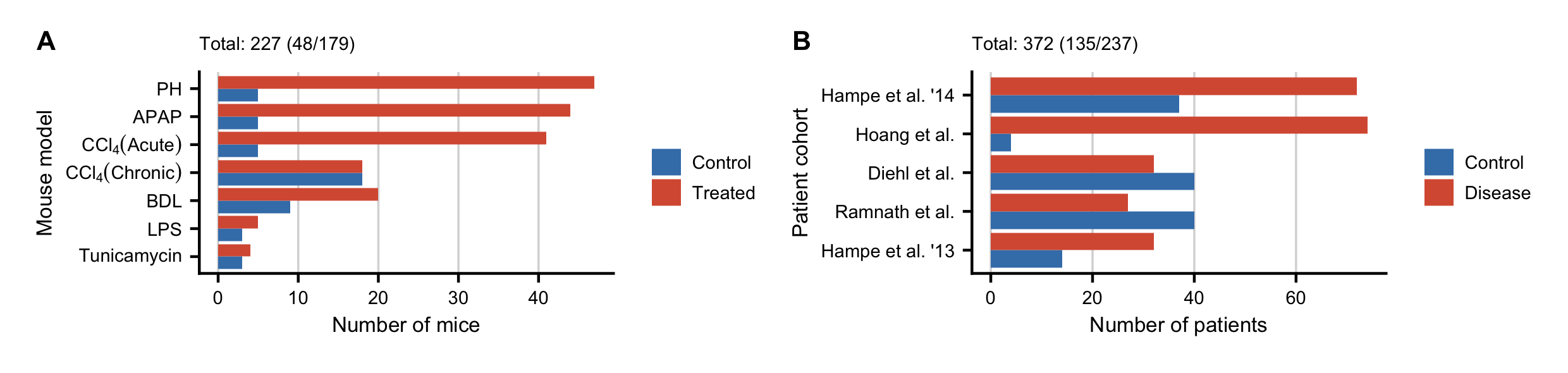
Figure C.1: Overview of the study cohorts. A. Number of analyzed mice per mouse model (control/treated). B. Number of analyzed patients per cohort (control/disease).

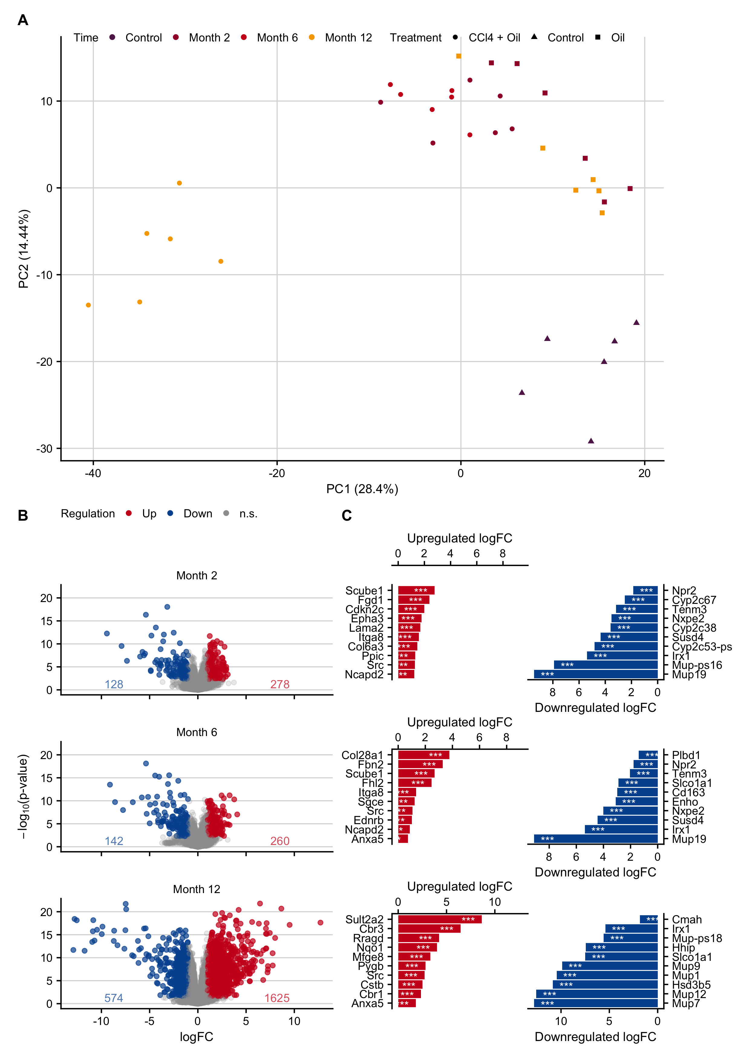
Figure C.2: Gene expression changes after induction of chronic liver damage in mice by repeated administration of 1 g/kg b.w. CCl₄ twice weekly for up to 12 months. A. PCA plot contextualized by time points and treatments. B. Volcano plots of months 2, 6 and 12. C. Genes with the highest log-fold changes.

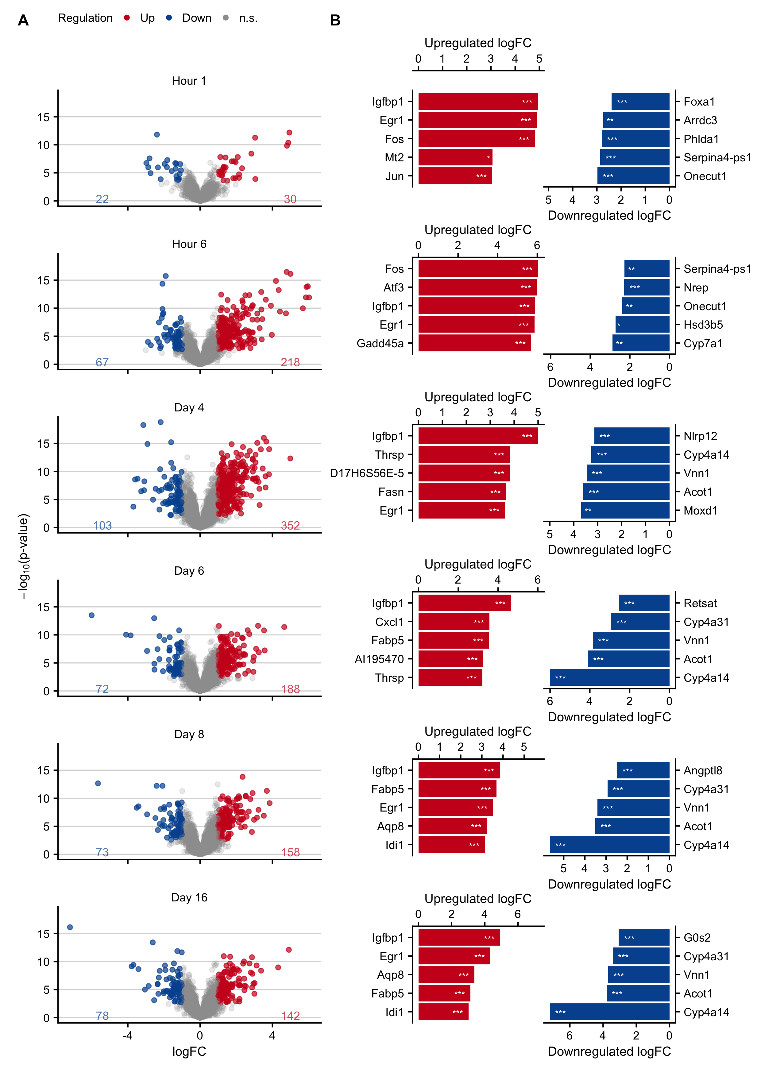
Figure C.3: Expression changes in an acute liver damage mouse model following a single administration of 300 mg/kg b.w. acetaminophen (APAP). A. Volcano plots at hours 1 and 6, and on days 4, 6, 8, 16 after APAP administration. B. Genes with the highest log-fold changes.

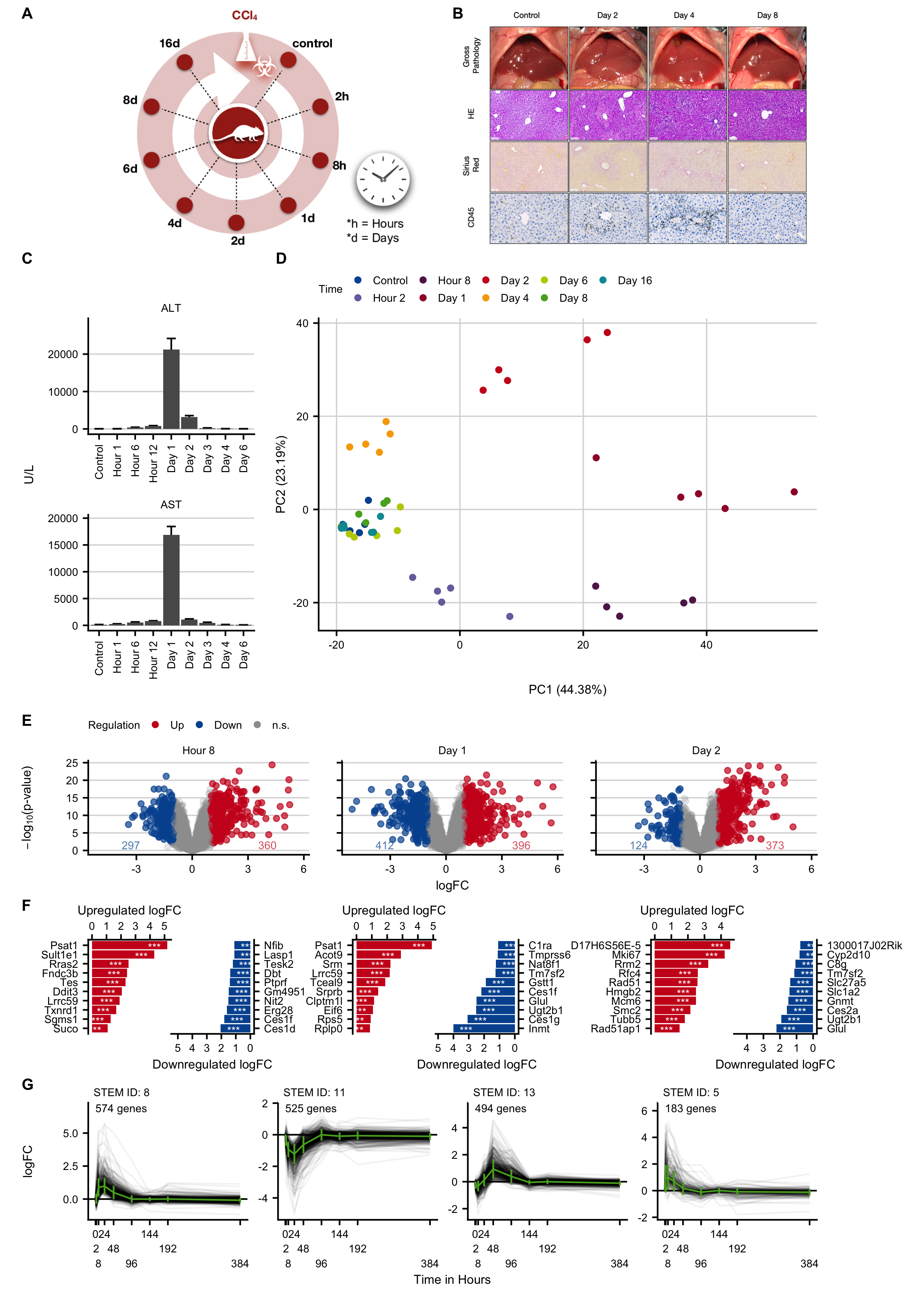
Figure C.4: Expression changes in an acute liver damage mouse model induced by administration of a single administration of CCl₄. A. Experimental design. B. Histological analysis with hematoxylin and eosin (HE) staining, fibrosis grade visualized by Sirius red, and infiltration of immune cells by CD45. The images show induction of pericentral liver lobule damage but without fibrosis development. Scale bars: 100 µm (HE; Sirius red) and 50 µm (CD45). C. Clinical chemistry with alanine transaminase (ALT), aspartate transaminase (AST) activities in plasma. D. PCA analysis of global expression changes. E. Volcano plots at12 hours, and on days 1 and 2 after CCl₄ administration. F. Genes with the highest log-fold changes. G. Time-resolved clustering of deregulated genes. The panels B and C were provided by Ahmed Ghallab.

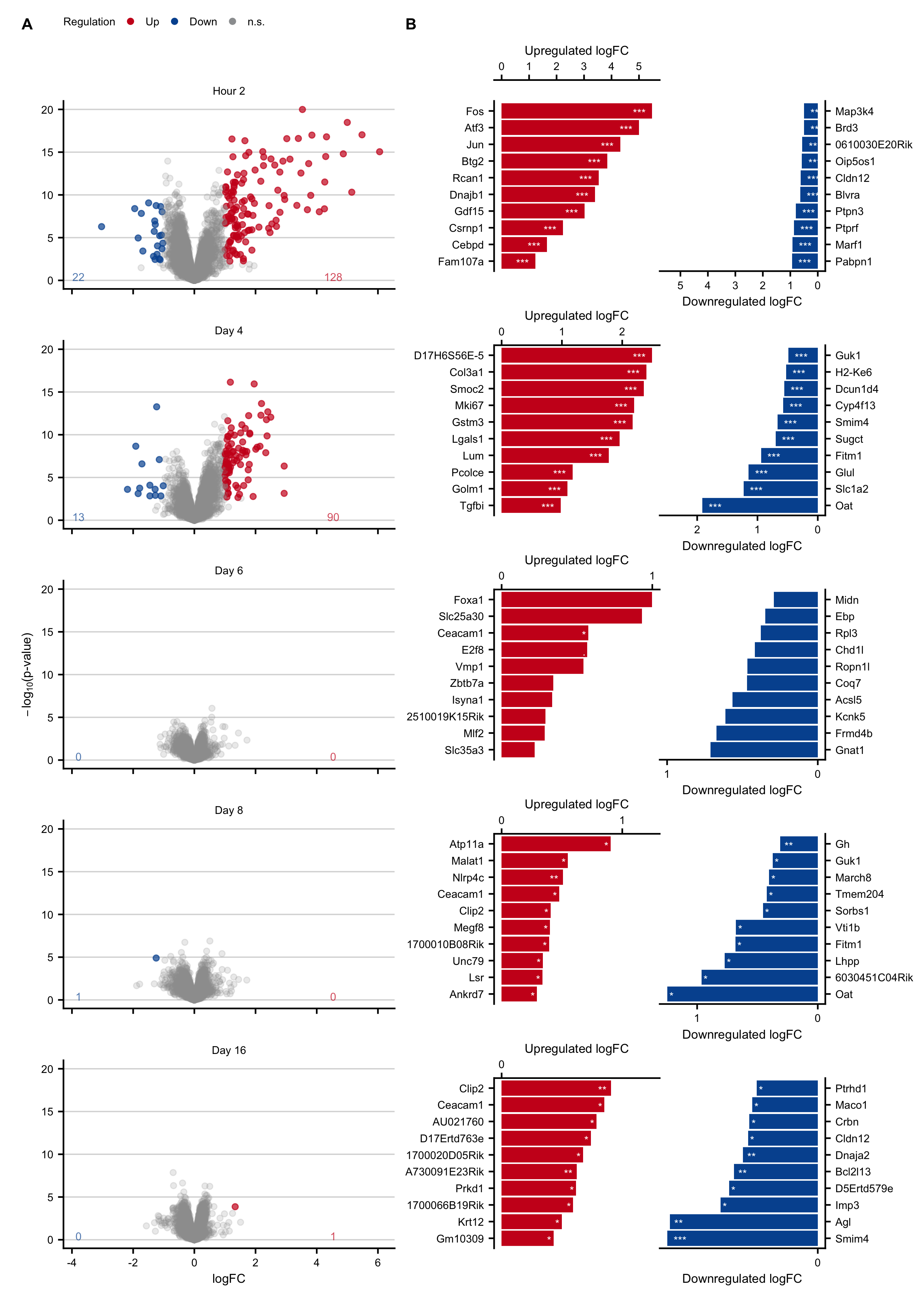
Figure C.5: Expression changes in an acute liver damage mouse model following a single administration of CCl₄. A. Volcano plots at 2 hours and on days 4, 6, 8, 16 after CCl₄ administration. B. Genes with the highest log-fold changes.

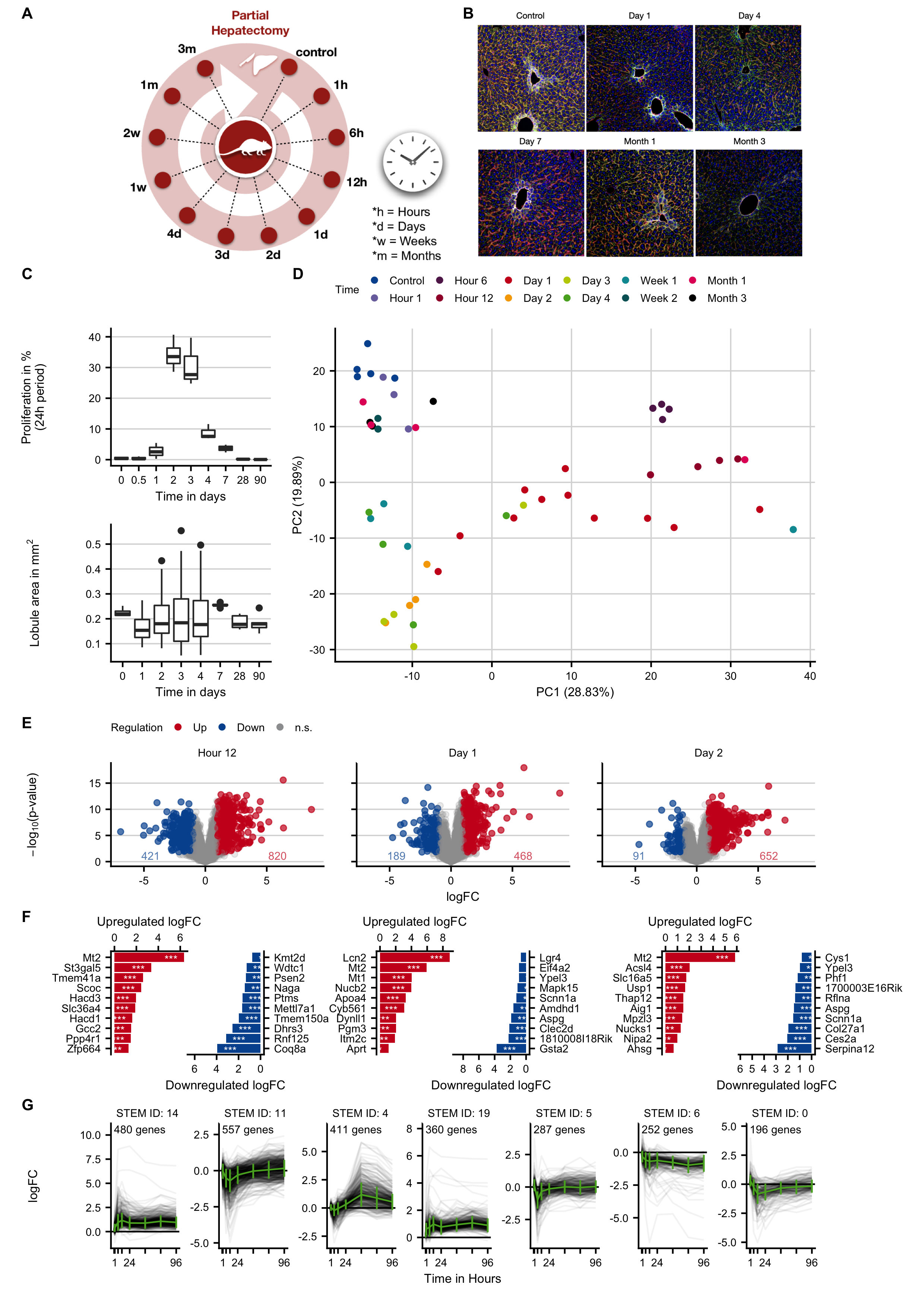
Figure C.6: Characterization and expression changes of mouse liver tissue after two-third hepatectomy. A. Experimental design. B. Transient increase in cell proliferation after hepatectomy based on BrDU staining and lobule area at different time periods after hepatectomy. C. Tissue morphology visualized by co-staining of bile canaliculi (DPPIV; green), pericentral hepatocytes (glutamine synthetase, white) and sinusoidal endothelial cells (yellow). D. PCA analysis of global expression changes. E. Volcano plots at 12 hours, and on days 1 and 2 after partial hepatectomy. F. Genes with the highest log-fold changes. G. Time-resolved clustering of deregulated genes. The panels B and C were provided by Ahmed Ghallab.

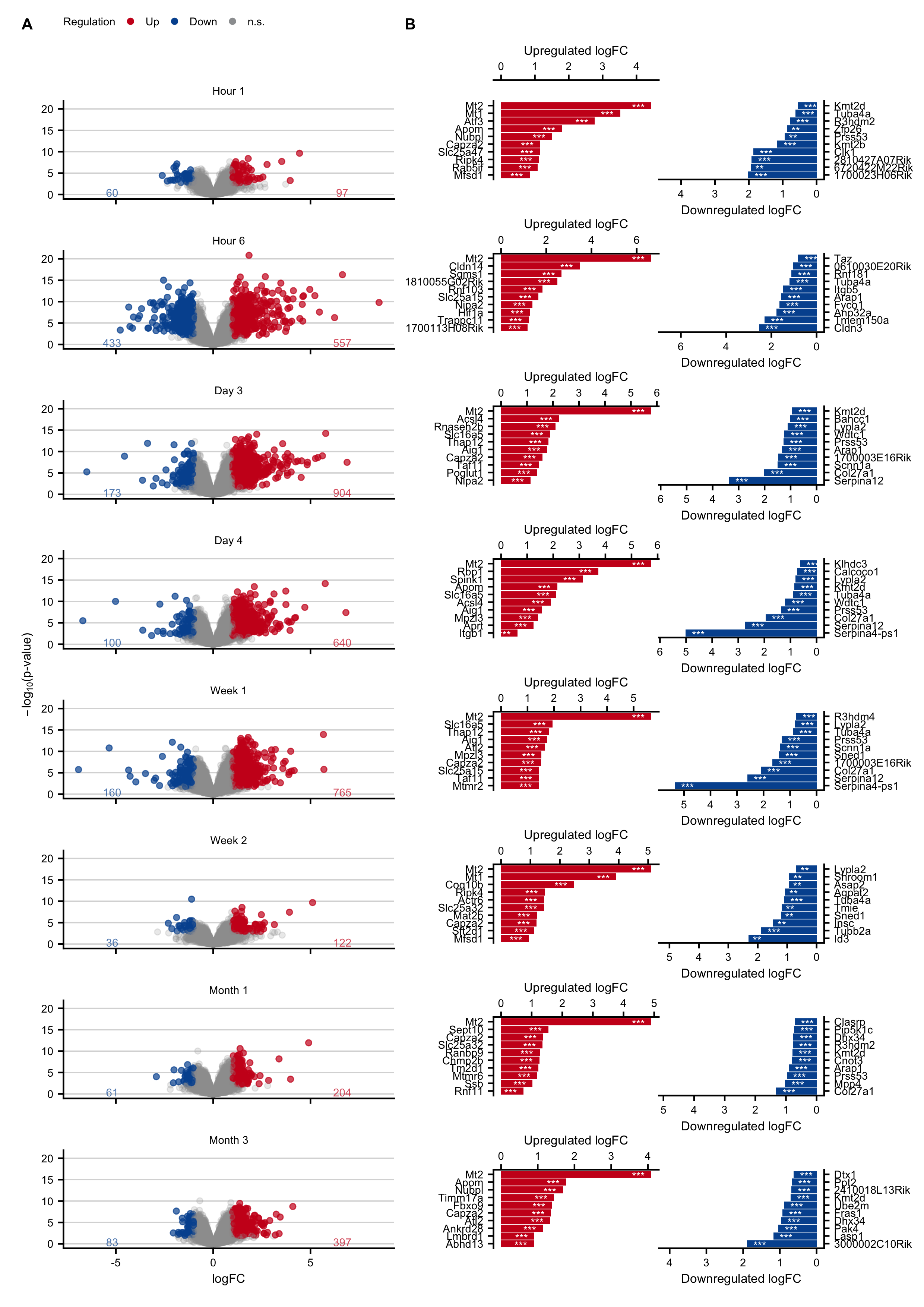
Figure C.7: Characterization and expression changes of mouse liver tissue after two-third hepatectomy. A. Volcano plots at hours 1 and 6, and on days 3 and 4, weeks 1 and 2, and months 1 and 3 after partial hepatectomy. B. Genes with the highest log-fold changes.

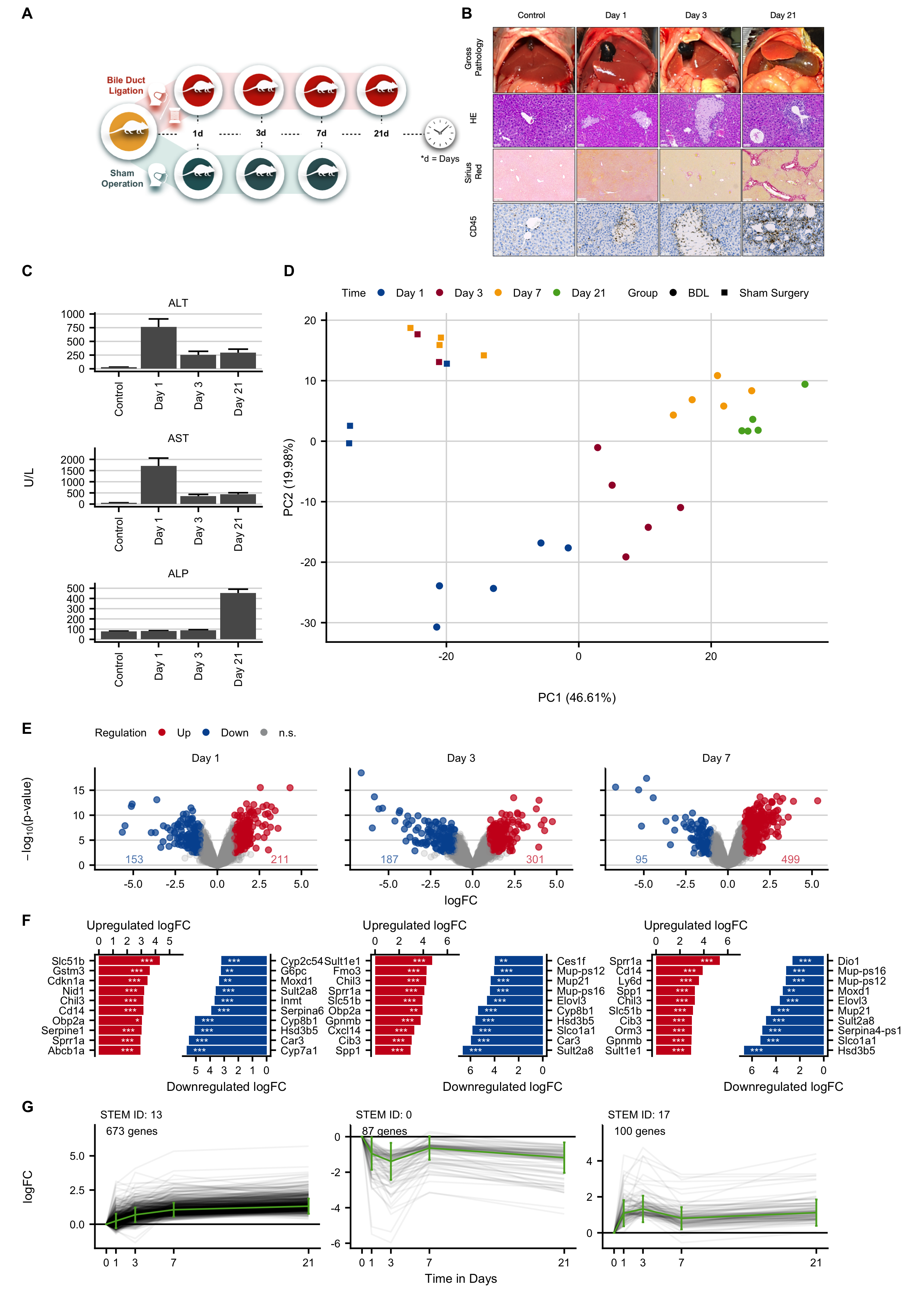
Figure C.8: Gene expression changes at different time intervals after induction of obstructive cholestasis by bile duct ligation (BDL). A. Experimental design. B. Histological analysis with hematoxylin and eosin (HE) staining, fibrosis grade visualized by Sirius red, and infiltration of immune cells by CD45. The images show bile infarct formation on days 1 and 3, and periportal fibrosis on day 21. Scale bars: 50 µm (HE; CD45) and 200 µm (Sirius red). C. Clinical chemistry with alanine transaminase (ALT), aspartate transaminase (AST) and alkaline phosphatase activities in plasma. D. PCA analysis of global expression changes. E. Volcano plots on days 1, 3 and 7 after BDL. F. Genes with the highest log-fold changes. G. Time-resolved clustering of deregulated genes. The panels B and C were provided by Ahmed Ghallab.

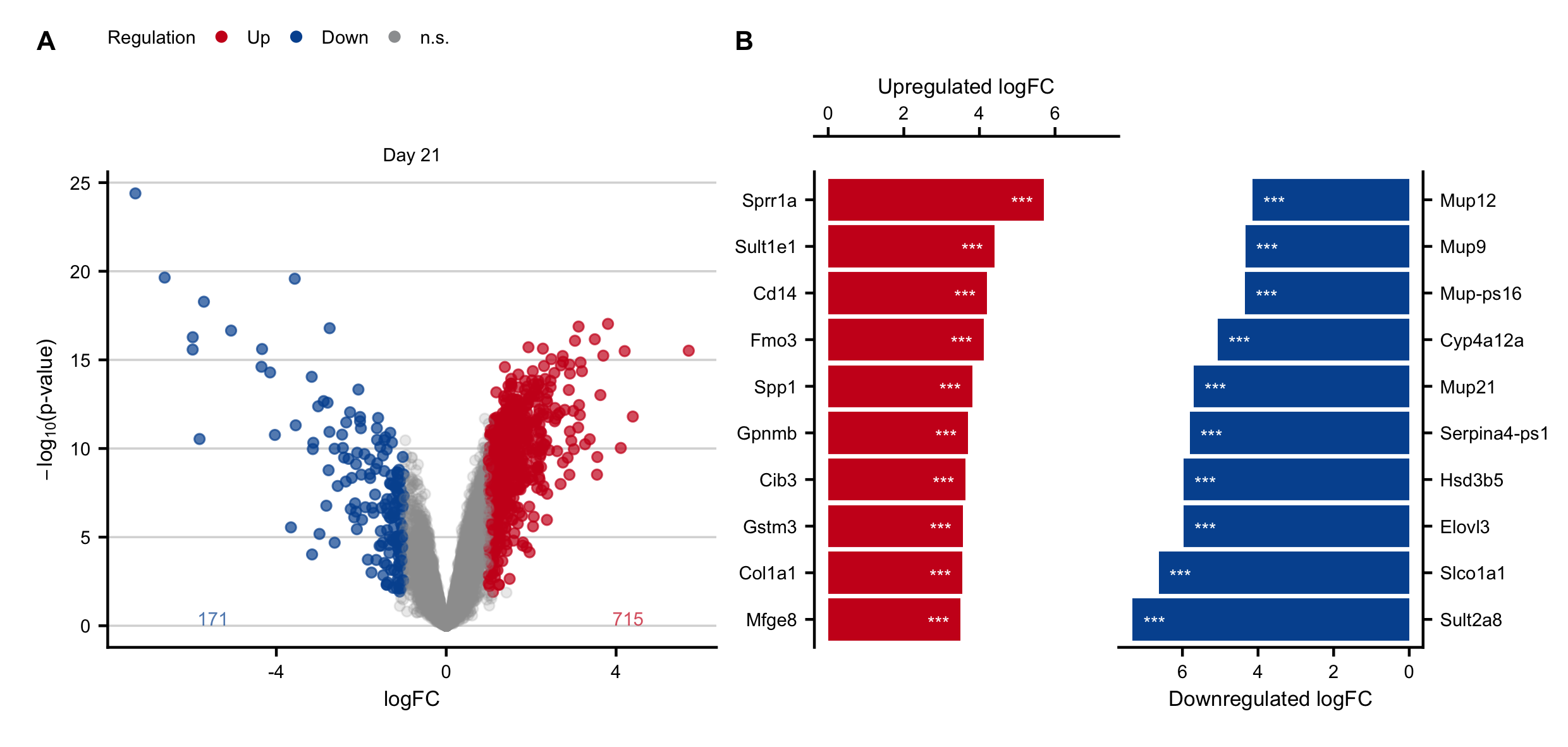
Figure C.9: Expression changes in the chronic stage after induction of obstructive cholestasis by bile duct ligation (BDL). A. Volcano plots on day 21 after BDL. B. Genes with the highest log-fold changes.

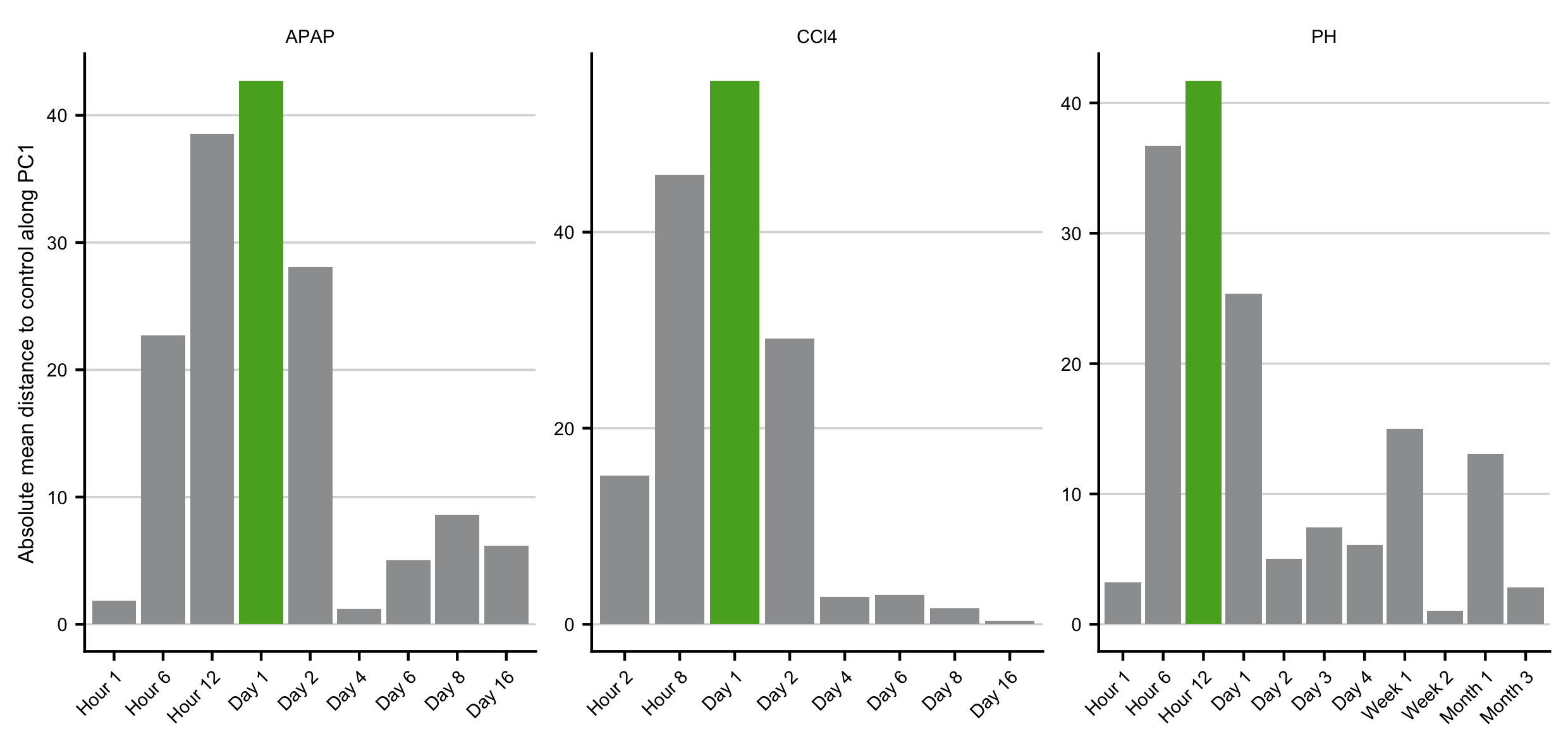
Figure C.10: Identification of the time point with the most deregulated expression profile after induction of acute liver injury based on the distance to the respective controls in PCA space along principle component 1 (PC1). Identified time point is colored in green.

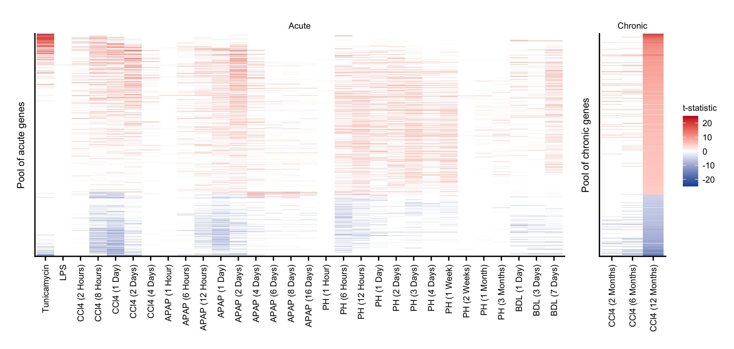
Figure C.11: Pool of unified acute and chronic genes demonstrating their respective consistent direction of regulation as indicated by t-statistic.

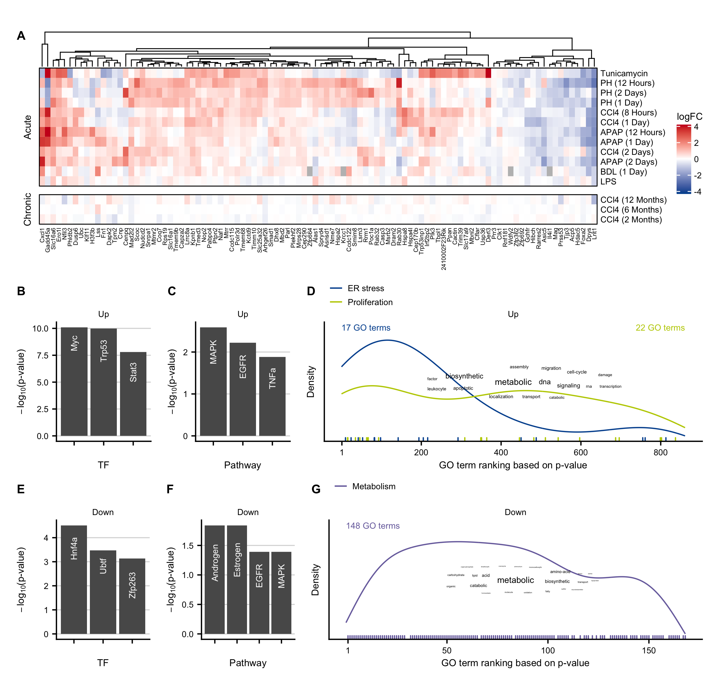
Figure C.12: Characterization of exclusive acute genes. A. Heatmap of top 100 exclusive acute genes. B-D. Overrepresented transcription factors identified by DoRothEA (B), pathways obtained by PROGENy (C), and GO terms (D) in the upregulated exclusive acute genes. E-F. Same as B-D but for the downregulated exclusive acute genes.

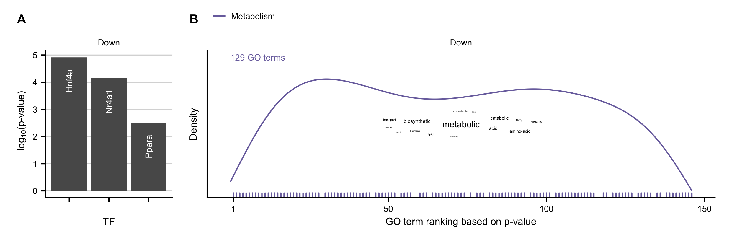
Figure C.13: A-B Overrepresented transcription factors identified by DoRothEA (A), and GO terms (B) in the set of commonly downregulated genes in acute and chronic mouse models.

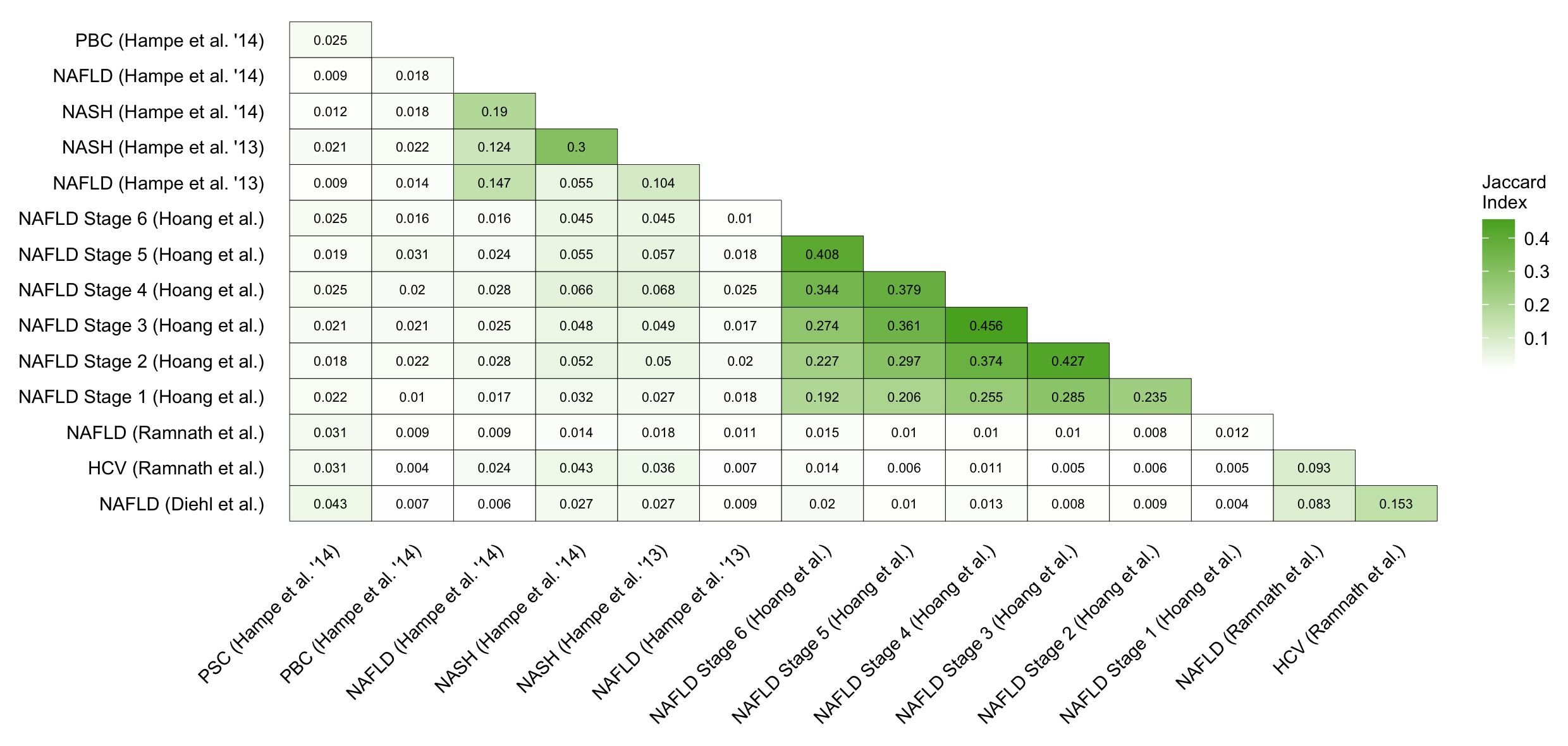
Figure C.14: Pairwise comparison of the similarity of the 500 deregulated genes per human contrast. Similarity is computed with the Jaccard index.

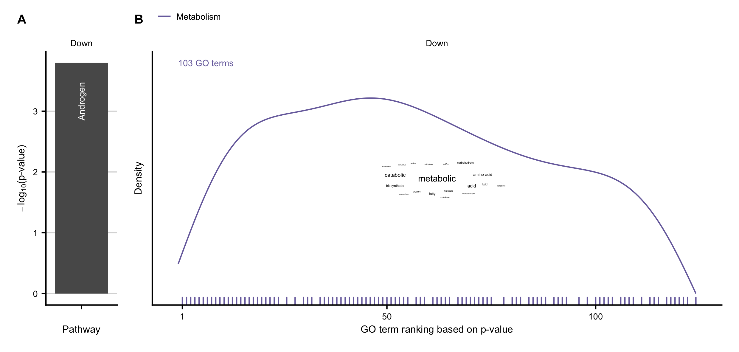
Figure C.15: A-B Overrepresented pathways obtained by PROGENy (A), and GO terms (B) in the set of consistently downregulated genes between human and mouse.

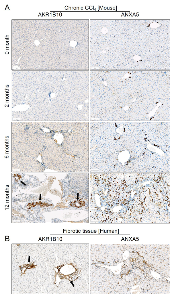
Figure C.16: Aldo-keto reductase (AKR1B10) and annexin V (ANXA5) increase in CLD of mice and humans. A. Immunostaining of AKR1B10 and ANXA5 at different stages during CLD progression induced by chronic CCl₄ administration in mice; AKR1B10 shows clusters of positive signals at 12 months (arrows); ANXA5 stained positive in the progressive ductular reaction. B. AKR1B10 and ANXA5 immunostaining in fibrotic tissues of human patients showing similar expression patterns as in mice. Scale bars: 100 µm. The entire figure was provided by Ahmed Ghallab.

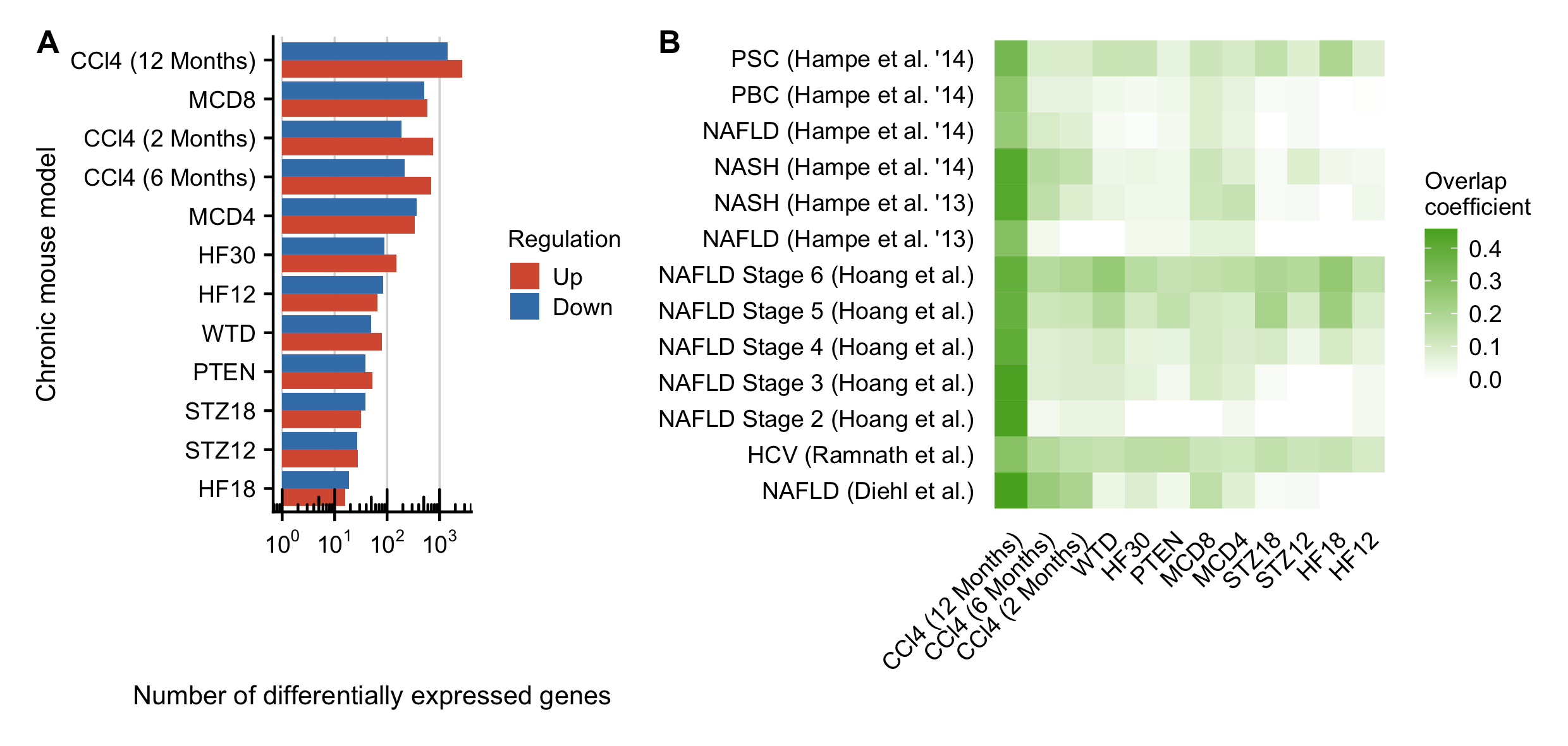
Figure C.17: A. Number of deregulated genes for the chronic CCl₄ mouse models complemented by 9 additional publicly available mouse models of chronic liver diseases. B Similarity of the significantly deregulated genes between all chronic mouse models and the human data. Similarity is computed as overlap coefficient.